Deep Q-Learning with PyTorch - Part 1

This is the first part of a series of three posts exploring deep Q-learning (DQN). DQN is a reinforcement learning algorithm that was introduced by DeepMind in their 2013 paper “Playing Atari with Deep Reinforcement Learning”. This first part will walk through a basic Python implementation of DQN to solve the cart-pole problem, using the PyTorch library. This initial implementation is based on the algorithm as described in the original paper. Over the next two parts we’ll ramp up the level of sophistication and end with a DQN implementation for the Atari game Breakout, that closely follows the details of DeepMind’s paper “Human-level control through deep reinforcement learning” which appeared in Nature in 2015.

This post is intended to compliment OpenAI’s “Spinning Up” which is an excellent resource if you have some familiarity with matrix operations, calculus and programming and want to get started with deep reinforcement learning. If a lot of the terminology here is new to you, I highly recommend reading through part one, part two and part three of their introduction to RL.

The problem

The environment that we’ll tackle in this first post is known as cart-pole. In particular, we’ll be using OpenAI’s implementation (CartPole-v0) from their Python library gym:

A pole is attached by an un-actuated joint to a cart, which moves along a frictionless track. The system is controlled by applying a force of +1 or -1 to the cart. The pendulum starts upright, and the goal is to prevent it from falling over. A reward of +1 is provided for every timestep that the pole remains upright. The episode ends when the pole is more than 15 degrees from vertical, or the cart moves more than 2.4 units from the center.
https://gym.openai.com/envs/CartPole-v0/

The environment is considered ‘solved’ when the average return (in this case the sum of rewards from each timestep) over 100 consecutive trials (episodes) for an agent is greater than or equal to 195.

States

Let’s take a moment to frame this problem more formally. Let’s first consider the state space $S$ (I will use the terms ‘states’ and ‘observations’ interchangably). The state space $S$ is a set whose elements describe all possible configurations of the environment. In part three we’ll modify our approach to use the rendered images of an environment to derive our observations. For now, however, we’ll focus on simply using the observations provided out-of-the-box by the gym library which essentially take the form of a 4-dimensional NumPy array of continuous-valued real numbers which have been wrapped in a custom Box class that gives us a few helper methods:

>>> import gym
>>> env = gym.make('CartPole-v0') # Instantiate the environment
>>> env.observation_space # Data structure used to hold env states
Box(4,)
>>> env.observation_space.sample() # Randomly sample a state
array([-0.01381209, -0.00833267, -0.04027887, -0.00729395])

These observation arrays have the following structure:

Index   Observation               Min                 Max
0       Cart Position             -4.8                4.8
1       Cart Velocity             -Inf                Inf
2       Pole Angle                -0.418 rad          0.418 rad
3       Pole Angular Velocity     -Inf                Inf

Actions

According to the description of the cart-pole environment above, the action space $A$ is discrete and contains two possible values.

>>> env.action_space
Discrete(2,)
>>> env.action_space.n # The size of the action space
2
>>> env.action_space.sample() # Randomly sample an action
1
>>> env.action_space.sample()
0

Note that $A = \{0, 1\}$ with 0 corresponding to a left action and 1 corresponding to a right action rather than -1 and 1 as in the description above.

Rewards

The cart-pole environment returns a reward of 1 for each action that results in the pole staying upright and the cart staying within a certain distance from the centre.

>>> env.reset() # Initialise an episode state
array([0.01337562, 0.02386517, 0.04556581, 0.01944452])
>>> observation, reward, done, info = env.step(1) # Perform action 1 (move right)
>>> reward
1
>>> done # Has the episode terminated?
False

For more details about gym environments/installation the official docs are a quick read.

The optimal action-value function $Q^*$

For a given envronment, the goal of RL is to choose a policy, that is, a function of the current state that selects the next action, that maximises the expected return of the agent that acts according to it. The policy could be represented by a probability distribution that is conditioned on a state $s_t$ at time $t$ that we then sample from. For DQN, and Q-learning more generally, policies are deterministic. That is, the action $a_t$ can be expressed as a function of the state $s_t$ at timestep $t$

Considering an episode of length $T$ timesteps, at each timestep $t$ we can define the future discounted return, which is a weighted sum of returns from the current timestep. If $\gamma$ is less than 1 then the contribution of future returns is discounted (a reward now is worth more than a reward later).

For a given state $s$ we can then define the optimal action-value function.

This gives us the expected future (discounted) return if we perform action $a$ when in a given state $s$ and then act according to the optimal policy from then on util the end of the episode.

Suppose for a moment that we had access to the true function $Q^* $ for a given environment with a finite set of actions, how would we use it? For a given state $s$ we could enumerate all the possible actions $(a_1, a_2, …, a_n)$, calculate $Q^* (s, a_i)$ and simply adopt a policy of choosing the action that maximises the expected return for the given state, setting $a = \max _a Q^* (s, a)$. The goal of Q-learning is to approximate the function $Q^*$ and adopt such a policy.

Note here that this depends on calculating Q for every action and therefore restricts this method to choosing actions for environments with discrete action spaces.

Approximating the $Q^*$ function

In order to approximate $Q^* $ we’ll be using a feedfoward neural network \(Q \approx Q^*\). The structure of this network and implementation details are discussed in detail below, but for now we’ll treat it as a single-valued function of two variables, $s$ and $a$, with parameters $\theta$.

In order to train the network we need (i) some targets and (ii) some kind of loss function. Rather that minimising a single loss function, however, we are going to minimise a sequence of loss functions where $i$ refers to the $i$th training step and $t$ is some timestep. Assume for a moment that we have access to a set of ‘experiences’ $\mathcal{D} = \lbrace e_1, e_2, …, e_n\rbrace$, where each element $e_i$ is a tuple of the form $e_i = (s_t, a_t, r_t, s_{t+1})$. Here, $s_t$ is a state at timestep $t$, $a_t$ is the action that was performed, $r_t$ is the observed reward and $s_{t+1}$ is the next state return by the environment. The loss functions then take the form

Where

Here $\theta^-$ refers to the fixed parameters of $Q$ at training step $i$. This can be thought of as a separate network whose parameters are not updated as part of the optimisation step. It turns out that it is possible to make the DQN procedure more stable by keeping theses ‘target network’ parameters fixed over a greater number of timesteps, which we’ll explore in the next post. At each training step the expectation above is approximated using minibatches and the parameters $\theta_i$ are updated via stochastic gradient descent.

NOTE: The original paper gives $y_i$ as an expectation w.r.t. to the environment state distribution. Since cart-pole is deterministic this will be equal to the expression for $y_i$ above.

Explicitly, since we are using the sample mean to approximate the expectation, we have

The expression $ r_t + \gamma \max_{a’} Q(s_{t+1}, a’; \theta^-) - Q(s_j, a_j; \theta_i) $ gives us the difference between the actual observed reward $r_t$ plus our estimate of the remainder of the Q* function when selecting optimal actions and our predeiction of the whole thing.

Now here we’re using some observation $s_t$, a reward $r_t$, an action $a_t$ and the following state $s_{t+1}$, but where are we drawing these from? A key idea that was introduced in the original DQN paper from DeepMind is that of an experience replay buffer. The experiences will be accumulated as we train and stored in a fixed-length buffer that we will then randomly sample from to generate the minibatches. More details are provided below, but essentially there will be a period of exploration where random actions are chosen and then a period where we become increasingly dependent on our learned $Q$ network to pick actions. After a number of timesteps most of the actions in the buffer will be generated by performing actions that maximise the output of the $Q$ network.

Random sampling of experiences to construct minibatches is important since it decorrelates samples resulting in less variance in parameter update steps. Also, if we were to select a consecutive sequence of experiences to perform the optimisation step, then current weights might currently bias the agent to always choose a left action, for example. The optimisation step would then nudge the parameters to make such actions more likely in future and could result in a viscous feedback loop.

NOTE: It is worth mentioning that DQN can be adapted for environments with continuous action spaces, where it goes by the name Deep Deterministic Policy Gradient (DDPG). The principal modification here is the introduction of a function that chooses an action that maximises Q which is learned as part of the training process.

The complete algorithm

Our implementation will closely follow the DQN algorithm as described in Vlad Mnih et al.’s 2013 paper “Playing Atari with Deep Reinforcement Learning”. Although the authors focused on a high-dimensional observation space which consisted of processed images of the Atari games, we’ll work our way up to this environment over these three posts and stick for now to the cart-pole environment and the 4-D observations that OpenAI’s gym implementation provides us with.

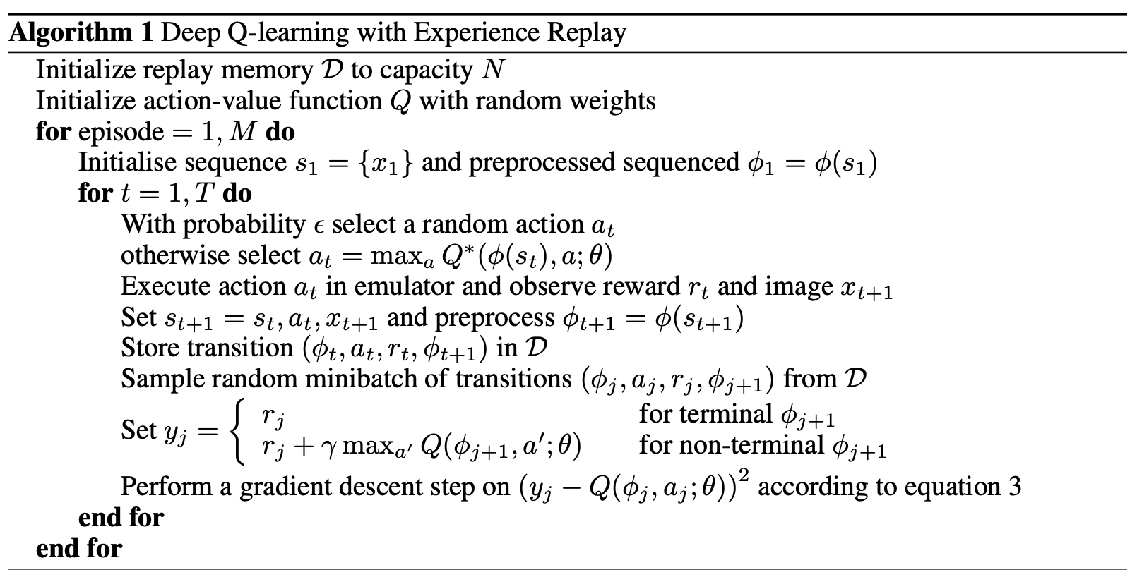
Note that the implementation described here will deviate from this in a few minor details. Firstly, rather than iterating over a fixed number of episodes and timesteps for each episode, we’ll simply iterate over a fixed number of timesteps. We’ll update the weights of our $Q$ network after every timestep, after an initial exploration period specified by learning_starts. The dqn function will exit when the environment when we have reached an average return of > 195 over 100 consecutive episodes or we reach the specified number of timesteps.

Secondly, the authors of the paper perform some preprocessing over a sequence of images to form a fixed-size representation of their environment’s states using some function $\phi_t = \phi(s_t)$. We will use the states $s_t$ from the cart-pole environment as-is for now (we can ignore the setting of $s_t = s_t, a_t, x_{t+1}$ too; these details will be addressed in the next post).

Implementation

A complete implementation is given below. We first define a few helper functions for generating our Q network (ffnn, which I pinched from the ‘Simplest Policy Gradient’ implementation in part three of ‘Spinning Up’), choosing the optimal action according to our Q network (best_action) and computing the loss (compute_loss). The rest of the code more-or-less devoted to implementing the dqn function that takes care of the complete DQN training process as described above.

The algorithm uses an $\epsilon$-greedy policy which means that it’ll randomly sample an action from the action space with probability $\epsilon$ or otherwise choose the best action from the current approximation of $Q^* $ (with probability 1 - $\epsilon$). The value of $\epsilon$ essentially controls the degree to which the agent will explore the environment vs the degree to which it will exploit its current ability to maximise its expected return. When we start training our agent, our $Q$ network is unlikely to provide a reasonable approximation of $Q^* $. In order to discover which actions lead to a higher accumulation of rewards over time we opt for an initial period of data collection via random actions. Hopefully some of these random actions will have resulted in a high return over some of the episodes and so training our network will nudge the weights of our $Q$ network to predict a higher value (expected return) under those circumstances if we follow the high-return actions.

After the initial exploration period, the implementation below begins to linearly decay the value of $\epsilon$ so that more and more of the agent’s actions are those which the $Q$ network predicts will maximise our reward. While $Q$ it may still not be a particularly good approximation of $Q^* $, it is hoped that it provides some reasonable estimates under some circumstances and then by mixing in some further random exploration we will gradually nudge the weights to push the average episode return up even more.

Some of the hyperparameters (learning rate, network size, batchsize) were taken from the DQN implementation in the Stable Baselines repo and seem to work well over a range of random seeds (see below for experimental results).

import argparse  # Command line argument parsing
import random

# Use a queue with a max length for the experience replay
# buffer (appending to it after it reaches its size limit
# will throw out the old ones)
from collections import deque

import gym
import numpy as np

import torch
from torch import nn
from torch.distributions.categorical import Categorical


def ffnn(sizes, activation=nn.Tanh, output_activaton=nn.Identity):
    # Build a feedforward neural network
    layers = []
    for j in range(len(sizes) - 1):
        act = activation if j < len(sizes) - 2 else output_activaton
        layers += [nn.Linear(sizes[j], sizes[j + 1]), act()]
    return nn.Sequential(*layers)


def best_action(q_func, obs):
    # Return tensors consisting of best actions and the corresponding
    # q_func values for each observation in the obs tensor
    with torch.no_grad():
        val, best_act = q_func(obs).max(1)
    return best_act, val


def dqn(
    timesteps=50000,
    bs=32,
    hidden=[64, 64],  # Hidden layer size in the Q approximator network
    replay_buffer_len=10000,
    lr=5e-4,
    epsilon_start=1,  # Starting value of epsilon
    epsilon_end=0.02,  # Final value of epsilon after annealing
    epsilon_decay_duration=2500,  # Anneal the value of epsilon over this many timesteps
    learning_starts=1000,  # Start training our Q approximation after this many timesteps
    gamma=0.99,  # Discount factor when computing returns from rewards
    train_freq=1,
    seed=42,
    render_every=0,  # Render every <render_every> episodes
    save=None  # Provide a filename here to save the final model to
):
    # Instantiate environment
    env = gym.make('CartPole-v0')

    # Set random seeds
    env.seed(seed)
    torch.manual_seed(seed)
    random.seed(seed)
    np.random.seed(seed)
    env.action_space.seed(seed)

    # Construct our Q network that we'll use to approximate Q*
    n_acts = env.action_space.n
    obs_size = env.observation_space.shape[0]

    # We're using a network that estimates Q* for each action
    # (corresponding to each output)
    q_net = ffnn([obs_size] + hidden + [n_acts])

    # Use Adam for our optimizer
    optimiser = torch.optim.Adam(q_net.parameters(), lr=lr)

    def epsilon_schedule(t, timesteps):
        # We'll use a linear decay function here
        eps = epsilon_start * (-t / timesteps + 1)
        eps = max(eps, epsilon_end)
        return eps

    # Initialise the experience replay buffer.
    # When the replay buffer reaches the max length discard oldest items
    # so we don't exceed the max length
    xp_replay = deque([], maxlen=replay_buffer_len)

    # Create some empty buffers for tracking episode-level details.
    # These will be used for logging and determining when we've finished.
    ep_returns = []
    rews = []  # Track rewards for each timestep and reset at end of episode

    ep_done = False
    loss = None
    obs = env.reset()

    for i in range(timesteps):
        should_render = len(
            ep_returns) % render_every == 0 if render_every else False
        if should_render:
            env.render()

        # Sample an action randomly with prob (1 - epsilon)
        eps = epsilon_schedule(i, epsilon_decay_duration)

        if random.random() < eps:
            act = env.action_space.sample()
        else:
            act = best_action(q_net,
                              torch.as_tensor([obs],
                                              dtype=torch.float32))[0].item()

        # Perform the action in the envrionment and record
        # an experience tuple
        obs_next, rew, ep_done, _ = env.step(act)

        # CartPole-v0 returns a reward of 1 for terminal states, most of which will
        # correspond to bad actions. Manually set to 0 for terminal states.
        rew = 0 if ep_done else rew
        xp = (obs.copy(), act, rew, obs_next.copy(), ep_done)

        rews.append(rew)
        xp_replay.append(xp)

        # Make sure we update the current observation for the next iteration!
        obs = obs_next

        if ep_done or i == timesteps - 1:
            ret = sum(rews)
            ep_returns.append(ret)

            num_episodes = len(ep_returns)

            # Cartpole is considered solved when the average return is >= 195
            # over 100 consecutive trials, let's stop training when we reach this
            # during our training.
            if num_episodes >= 100 and np.mean(ep_returns[-100:]) >= 195:
                print(f'DONE! timesteps: {i} \t episodes: {num_episodes}')
                torch.save(q_net.state_dict(), save)
                return ep_returns

            ep_returns.append(sum(rews))
            rews = []

            obs = env.reset()

        if i >= learning_starts and i % train_freq == 0:
            # Sample from our experience replay buffer and update the parameters
            # of the Q network
            minibatch = random.sample(xp_replay, min(bs, len(xp_replay)))

            mb_obs = []
            mb_acts = []
            mb_rews = []
            mb_obs_next = []
            mb_done = []

            # Construct the targets and inputs for our loss function
            for obs_, act, rew, obs_next_, done in minibatch:
                mb_obs.append(obs_)
                mb_acts.append(act)
                mb_rews.append(rew)
                mb_obs_next.append(obs_next_)
                mb_done.append(0 if done else 1)

            mb_obs = torch.as_tensor(mb_obs, dtype=torch.float32)
            mb_obs_next = torch.as_tensor(mb_obs_next, dtype=torch.float32)
            mb_rews = torch.as_tensor(mb_rews, dtype=torch.float32)
            mb_done = torch.as_tensor(mb_done, dtype=torch.float32)
            mb_acts = torch.as_tensor(mb_acts)

            optimiser.zero_grad()

            # Create the target vals y_i for our loss function
            with torch.no_grad():
                y = mb_rews + gamma * mb_done * best_action(
                    q_net, mb_obs_next)[1]

            # Perform a gradient descent step on (y_i - Q(s_i, a_i)
            x = q_net(mb_obs)[torch.arange(len(mb_acts)), mb_acts]
            loss = ((y - x)**2).mean()

            # Compute gradients and update the parameters
            loss.backward()
            optimiser.step()

        num_episodes = len(ep_returns)

        if num_episodes % 100 == 0 and ep_done:
            print(
                f'episodes: {num_episodes} \t timestep: {i} \t epsilon: {eps}' \
                    f'\t last loss: {loss}' \
                        f'\t return (last 100): {np.mean(ep_returns[-100:])}'
            )
    return ep_returns


if __name__ == '__main__':
    parser = argparse.ArgumentParser()
    parser.add_argument('--timesteps', type=int, default=50000)
    parser.add_argument('--bs', type=int, default=32)
    parser.add_argument('--replay-buffer-len', type=int, default=10000)
    parser.add_argument('--lr', type=float, default=5e-4)
    parser.add_argument('--epsilon-start', type=float, default=1.0)
    parser.add_argument('--epsilon-end', type=float, default=0.02)
    parser.add_argument('--epsilon-decay-duration', type=int, default=2500)
    parser.add_argument('--learning-starts', type=int, default=1000)
    parser.add_argument('--seed', type=int, default=42)
    parser.add_argument('--render-every', type=int, default=0)
    args = parser.parse_args()

    dqn(
        timesteps=args.timesteps,
        bs=args.bs,
        replay_buffer_len=args.replay_buffer_len,
        lr=args.lr,
        epsilon_start=args.epsilon_start,
        epsilon_end=args.epsilon_end,
        epsilon_decay_duration=args.epsilon_decay_duration,
        learning_starts=args.learning_starts,
        seed=args.seed,
        render_every=args.render_every,
    )

Details

The results are shown below in the next section if you fancy skipping ahead, but I’ve included a more detailed walkthrough here of some of the sections of the above code to help it sink in. As usual, learning an algorithm is best done by implementing it oneself but hopefully this example will be of some use and maybe help a weary traveller if they get stuck. In the following section I’m going to assume you’re familiar with neural networks, or at least the idea of linear functions/matrix operations.

Q-network initialisation

I borrowed the feed-foward neural network initialisation code from OpenAI’s ‘Simplest Policy Gradient’ implementation in part three of ‘Spinning Up’. The function takes a list of sizes and returns a neural network with an input size of length size[0], ‘hidden layers’ of sizes sizes[1], sizes[2], ..., sizes[-2] and a final output layer of size sizes[-1]. The non-linearity that we’ll use for the hidden layers is specified by the activation argument, and the one for the output layer is specificed by the output_activation argument. We’ll drill down a bit into what all this means exactly.

def ffnn(sizes, activation=nn.Tanh, output_activaton=nn.Identity):
    # Build a feedforward neural network
    layers = []
    for j in range(len(sizes) - 1):
        act = activation if j < len(sizes) - 2 else output_activaton
        layers += [nn.Linear(sizes[j], sizes[j + 1]), act()]
    return nn.Sequential(*layers)

The neural network that we use in the DQN implementation is instantiated by q_net = ffnn([obs_size] + hidden + [n_acts]). Where obs_size is 4 (the size of the observation vector returned from the environment when env.step is called), hidden is the list [64, 64], and n_acts is 2 (corresponding to the left 0 and right 1 actions that the environment uses). This defines a function

We can decompose this function into it’s constituent parts (functions) that make it into a neural network. The following shows the chain of transformations that our input vector is going to go through as it’s minced into its final state.

More explictly in terms of the operations being performed, if we have three linear functions $L_1 : \mathbb{R}^{4} \to \mathbb{R}^{64}$, $L_2 : \mathbb{R}^{64} \to \mathbb{R}^{64}$ and $L_3 : \mathbb{R}^{64} \to \mathbb{R}^{2}$. We can break the computation down to the following steps for a given input $x$, where we have

\(\tag{1} v_1 = L_1(x) + b_1\) \(\tag{2} v_2 = \tanh(v_1)\) \(\tag{3} v_3 = L_2(v_2) + b_2\) \(\tag{4} v_4 = \tanh(v_3)\) \(\tag{5} v_5 = L_3(v_4) + b_ 3\)

Step (1) converts the input into a vector with 64 components using $L_1$ and adds a bias term $b_1$ to it. Step (2) applies an element-wise $\tanh$ function whose output is the first hidden layer. Steps (3) and (4) repeat this process, this time using $L_2$. Finally in step (5) the output of our neural network is produced by applying $L_3$ to the second hidden layer, reducing it from a vector of size 64 to 2-vector.

The idea is that we represent the linear transformations using matrices and update the components of the matrix to minimise some loss function. PyTorch gives us a tensor library to allow us to perform quick numerical calculations using Python. A key feature of PyTorch is that tensors will record operations that have been performed on them and allow us to automatically compute the gradients of these operations with respect to the tensor components (our parameters) via back-propagation. The nn.Linear class will give us a such a tensor with the specified size, nn.Tanh gives us our non-linear $\tanh$ function and the nn.Sequential class will wrap up all these layers in a single object. We can then pass the returned object an input tensor and it will perform the complete computation while performing the necessary book-keeping to let us compute the gradient w.r.t. the parameters with a single method call!

>>> ffnn([4, 64, 64, 2])
Sequential(
  (0): Linear(in_features=4, out_features=64, bias=True)
  (1): Tanh()
  (2): Linear(in_features=64, out_features=64, bias=True)
  (3): Tanh()
  (4): Linear(in_features=64, out_features=2, bias=True)
  (5): Identity()
)

Note that the Linear class takes care of including an intercept term via the bias argument too.

The first matrix (2-D tensor) takes an input of size 4 and returns an output of size 64, so it has (4 x 64) + (1 x 64) parameters (the second pair of brackets is for the bias term). The second maps an input of size 64 to an output of size 64 so this one has (64 x 64) + (1 x 64) parameters. The third maps an input of size 64 to an output of size 2 which gives it (64 x 2) + (1 x 2) parameters. We therefore have a total of 4610 parameters in our neural network.

Why does our Q-network have two outputs?

In the code above we’ve used a neural network $Q(s; \theta) \mapsto (q_1, q_2)$ where $s$ is the current state of the environment and $(q_1, q_2)$ are the predicted action-values for the actions $0$ and $1$ respectively. For a more literal implementation of the above algorithm we could have instead made $Q$ a function of both the action and the state mapping to the estimated value for the pair, giving us an approximator of $Q^* $ in the familar form $Q(s, a; \theta) \mapsto q$.

The primary advantage, as far as I’m aware, of the given implementation is that in enables us to write a slightly more efficient (and cleaner-looking) function for choosing the best action for a given state. In order to find the best action we can simply retrieve the index of the highest output using a single forward pass. The alternative would require us to perform two passes to work out which action is best. In addition to this we would have to work a little bit more to construct the inputs by concatenating a one-hot representation of the action with the state before passing it in to the function.

def best_action(q_func, obs):
    # Return tensors consisting of best actions and the corresponding
    # q_func values for each observation in the obs tensor
    with torch.no_grad():
        val, best_act = q_func(obs).max(1)
    return best_act, val

A possible alternative:

def best_action(q_func, obs, n_acts):
    # Create n inputs for our Q net and choose the best action
    # Use one-hot encoding for actions and concatenate the observation:
    # obs = [o_1, o_2,..., o_k], n_acts = 2 give us two candidate inputs
    # for the Q function:

    # [1, 0, o_1, o_2,..., o_k], [0, 1, o_1, o_2,..., o_k]
    one_hot = torch.eye(n_acts)
    expanded_obs = torch.as_tensor([obs],
                                    dtype=torch.float32).expand(n_acts, -1)
    q_in = torch.cat((one_hot, expanded_obs), 1)
    best_act = torch.argmax(q_func(q_in)).item()
    return best_act

Inititalisation

Next let’s take a look at the first chunk of the dqn function.

As discussed earlier, we start off by instantiating the environment

 # Instantiate environment
env = gym.make('CartPole-v0')

We then set the random seeds everywhere that needs them so we can reproduce any experiements we run.

env.seed(seed)
torch.manual_seed(seed)
random.seed(seed)
np.random.seed(seed)
env.action_space.seed(seed)

RL algorithms have a reputation for being brittle. That is, small code modifications/randomness can result in dramatic changes in the performance of an agent. By fixing the random seed we can get a handle on the effect of any modifications we might make to the hyperparameters or algorithm itself. General performance improvements can then be measured over several random seeds by some sort of averaging. The variance of the performance in the simple cart-pole environment of our algorithm can be observed in the results section below. Sources of randomness in this case include generating the initial state of the environment, sampling minibatches from the experience replay buffer and initialising the weights in our neural network.

Next we’ll initialise the neural network (for more detail see the section above) and our optimiser. For our implementation we’ll use Adam to update the parameters of q_net. When we compute the loss function, we can then simply calculate the gradients using PyTorch. Calling optimiser.step(lr=learning_rate) will then perform the required update to the parameters in our network.

# Construct our Q network that we'll use to approximate Q*
n_acts = env.action_space.n
obs_size = env.observation_space.shape[0]

# We're using a network that estimates Q* for each action
# (corresponding to each output)
q_net = ffnn([obs_size] + hidden + [n_acts])

# Use Adam for our optimizer
optimiser = torch.optim.Adam(q_net.parameters(), lr=lr)

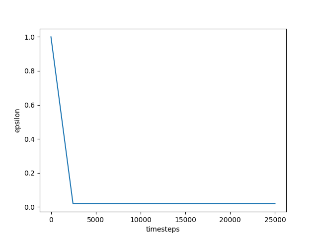
Next we define a function that will take care of our epsilon scheduling. In order to regulate the degree of exploration our agent will perform in the environment (where actions are chosen randomly instead of by using the $Q$ network), we will use a clamped linear decay function.

# Note: epsilon_start and epsilon_end are defined as parameters of dqn
def epsilon_schedule(t, timesteps):
    # We'll use a linear decay function here
    eps = epsilon_start * (-t / timesteps + 1)
    eps = max(eps, epsilon_end)
    return eps

In the main example above, epsilon will start at 1 until it reaches 0.02 over a period of 2500 timesteps (sepcified by the epsilon_decay_duration).

Finally, before kicking off the training the loop, we initialise some buffers to track ‘experience’ (corresponding to the $(\phi_t, a_t, r_t, \phi_{t+1})$ tuple in the algorithm description above), episode returns and rewards at each timestep during an episode. Here, the experience tuples will actually consist of $(s_t, a_t, r_t, s_{t+1}, d_t)$ where $s_t$ is the state of the environment at time $t$ and $d_t$ is a boolean value that records whether the state is terminal or not.

# Initialise the experience replay buffer.
# When the replay buffer reaches the max length discard oldest items
# so we don't exceed the max length
xp_replay = deque([], maxlen=replay_buffer_len)

# Create some empty buffers for tracking episode-level details.
# These will be used for logging and determining when we've finished.
ep_returns = []
rews = []  # Track rewards for each timestep and reset at end of episode

ep_done = False
loss = None
obs = env.reset()

The experience replay buffer xp_replay is a queue that truncates itself when it reaches maxlen, discarding the oldest elements.

We also keep track of the latest loss and episode state - ep_done will tell us when we should reset the ep_returns and rews buffers and the environment itself. We reset the environment and track our first observation.

The training loop - acting

Let’s look at the first part of the training loop.

for i in range(timesteps):
    should_render = len(
        ep_returns) % render_every == 0 if render_every else False

    if should_render:
        env.render()

    # Sample an action randomly with prob (1 - epsilon)
    eps = epsilon_schedule(i, epsilon_decay_duration)

    if random.random() < eps:
        act = env.action_space.sample()
    else:
        act = best_action(q_net,
                            torch.as_tensor([obs],
                                            dtype=torch.float32))[0].item()

    # Perform the action in the envrionment and record
    # an experience tuple
    obs_next, rew, ep_done, _ = env.step(act)

    # CartPole-v0 returns a reward of 1 for terminal states, most of which will
    # correspond to bad actions. Manually set to 0 for terminal states.
    rew = 0 if ep_done else rew
    xp = (obs.copy(), act, rew, obs_next.copy(), ep_done)

    rews.append(rew)
    xp_replay.append(xp)

    # Make sure we update the current observation for the next iteration!
    obs = obs_next

The first part takes care of the rendering. len(ep_returns) gives us the number of episodes we’ve run, so if this agrees with the render frequency (given by render_every), we want to display the current state of the environment.

should_render = len(
        ep_returns) % render_every == 0 if render_every else False

if should_render:
    env.render()

The next few lines make use of the epsilon_schedule function that we discussed earlier.

# Sample an action randomly with prob (1 - epsilon)
eps = epsilon_schedule(i, epsilon_decay_duration)

if random.random() < eps:
    act = env.action_space.sample()
else:
    act = best_action(q_net,
                        torch.as_tensor([obs],
                                        dtype=torch.float32))[0].item()

Here we’re drawing uniformly distributed random number from the range 0 and 1 using random.random(). eps $\times 100$ % of the time this value will be less than eps, and when it is let’s sample a random action. When it is not, let’s choose the best action as predicted by our q_net.

Next we peform the chosen action in the environment and construct the tuple for the experience replay buffer.

# Perform the action in the envrionment and record
# an experience tuple
obs_next, rew, ep_done, _ = env.step(act)

# CartPole-v0 returns a reward of 1 for terminal states, most of which will
# correspond to bad actions. Manually set to 0 for terminal states.
rew = 0 if ep_done else rew
xp = (obs.copy(), act, rew, obs_next.copy(), ep_done)

rews.append(rew)
xp_replay.append(xp)

# Make sure we update the current observation for the next iteration!
obs = obs_next

The training loop - handling complete episodes

When an epsiode is complete we want to check if our solve condition is met. The solve condition in this case is an episode length (corresponding to the sum of rewards) greater than or equal to 195. If the episode is not complete we we’ll update the buffers and reset the obs value. If we hit the maximum number of timesteps specified we’ll check if we’re done just in case the in-progress epsiode has resulted in us reaching the solve condition.

if ep_done or i == timesteps - 1:
    ret = sum(rews)
    ep_returns.append(ret)

    num_episodes = len(ep_returns)

    # Cartpole is considered solved when the average return is >= 195
    # over 100 consecutive trials
    if num_episodes >= 100 and np.mean(ep_returns[-100:]) >= 195:
        print(f'SOLVED! timesteps: {i} \t episodes: {num_episodes}')
        return ep_returns

    ep_returns.append(sum(rews))
    rews = []

    obs = env.reset()

The training loop - updating model parameters

After a period of learning_starts timesteps we want to start updating the model parameters every train_freq timesteps.

if i >= learning_starts and i % train_freq == 0:
    # Sample from our experience replay buffer and update the parameters
    # of the Q network
    minibatch = random.sample(xp_replay, min(bs, len(xp_replay)))

    mb_obs = []
    mb_acts = []
    mb_rews = []
    mb_obs_next = []
    mb_done = []

    # Construct the targets and inputs for our loss function
    for obs_, act, rew, obs_next_, done in minibatch:
        mb_obs.append(obs_)
        mb_acts.append(act)
        mb_rews.append(rew)
        mb_obs_next.append(obs_next_)
        mb_done.append(0 if done else 1)

    mb_obs = torch.as_tensor(mb_obs, dtype=torch.float32)
    mb_obs_next = torch.as_tensor(mb_obs_next, dtype=torch.float32)
    mb_rews = torch.as_tensor(mb_rews, dtype=torch.float32)
    mb_done = torch.as_tensor(mb_done, dtype=torch.float32)
    mb_acts = torch.as_tensor(mb_acts)

    optimiser.zero_grad()

    # Create the target vals y_i for our loss function
    with torch.no_grad():
        y = mb_rews + gamma * mb_done * best_action(
            q_net, mb_obs_next)[1]

    # Perform a gradient descent step on (y_i - Q(s_i, a_i)
    x = q_net(mb_obs)[torch.arange(len(mb_acts)), mb_acts]
    loss = ((y - x)**2).mean()

    # Compute gradients and update the parameters
    loss.backward()
    optimiser.step()

The first part simply samples a minibatch-size number (or whatever we have if we haven’t accumulated enough elements yet) of elements from the experience buffer xp_replay. We then iterate through the elements and create PyTorch tensors for the elements at each index of the sampled experience tuples. That is, if you imagine stacking the tuples on top of each other vertically, the mb_* tensors would be the resulting columns.

Next we use optimiser.zero_grad() to set any accumulated gradients to 0 before computing our loss function and calculating the required gradients. We then construct the targets for out loss function.

# Create the target vals y_i for our loss function
with torch.no_grad():
    y = mb_rews + gamma * mb_done * best_action(
        q_net, mb_obs_next)[1]

Notice that mb_done was set to 0 for terminal states and 1 otherwise. The above calculates

We use torch.no_grad() here so the network’s computational graph is not updated - these targets are treated like (fixed) observed values in supervised learning and so we won’t be taking this calculation into account when computing the gradients of the loss function w.r.t. the network parameters.

The next bit calculates the loss.

x = q_net(mb_obs)[torch.arange(len(mb_acts)), mb_acts]
loss = ((y - x)**2).mean()

The inputs for the loss function are computed using the q_net by plucking the predicted action-value for the given action. A neat thing about PyTorch tensors is that their elements can be accessed by lists of indices (in tensor form).

Evaluating a batch of observations of size 32 gives us 32 pairs of Q values, one for each action.

>>> q_net(mb_obs)
tensor([[-0.0236, -0.2143],
        [-0.1013, -0.2034],
        [-0.0256, -0.2069],
        [-0.0280, -0.2153],
        [-0.0623, -0.1981],
        [-0.0870, -0.1797], ... # len 32

We can then create a tensor of the Q values returned corresponding to each of the actions by passing in a list of column indices via torch.arange(len(mb_acts)) and row indices via mb_acts.

>>> torch.arange(len(mb_acts))
tensor([ 0,  1,  2,  3,  4,  5, ... # up to 31
>>> mb_acts
tensor([0, 0, 0, 0, 0, 1, ... # len 32
>>> q_net(mb_obs)[torch.arange(len(mb_acts)), mb_acts]
tensor([-0.0236, -0.1013, -0.0256, -0.0280, -0.0623, -0.1797, ...

Now that we have computed the loss, we can use backprop to calculate the gradients and update the parameters using the optimiser.

loss.backward()
optimiser.step()

Results

The results of running the dqn function over 10 random seeds are shown below. All runs demonstrate a ‘warm-up’ period, where the exploration typically takes place, followed period of sustained policy improvement. It is interesting to observe, however, the variance in performance during training, with some policies degrading significantly in performance before reaching the 195 episode threshold.

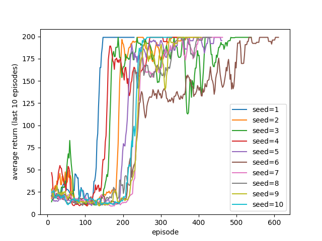
Here’s one of the trained agents

What’s next?

In the next part we’ll add a few bells and whistles to our DQN code before ramping up the neural network to handle Atari environment inputs in part three.